Supply chain network design (SCND) is a powerful tool for improving business operations. Optimization and simulation are the two main branches of SCND.
Optimization accounts for over 90% of all work that is being done by SCND teams. It can be used to solve a wide variety of supply chain problems. But it has gaps. Simulation techniques can fill those gaps and allow for a more holistic view of a company’s supply chain. This article describes how to incorporate simulation techniques into optimization, build a stochastic optimization model, and end up with a more resilient supply chain model.
Demand is at the Heart of Supply Chain Network Design
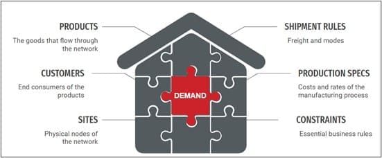
The first step in the SCND process is translating business rules into a set of data inputs: demand, products, customers, sites, shipment rules, production details, and various constraints. Assumptions around demand are in the center here because, unlike all other main components, they are the most difficult to forecast.

SCND team’s first goal is to build a baseline model that represents the current state of the business. After that the team works in an iterative way, answering stakeholder’s questions regarding how the network will react to various changes (e.g. what if a recession hits next year? What if we experience a storm? What if the new product’s sales take off faster than we expect?)
As the SCND team prepares to tackle these questions, they can approach it from different angles.
One possible approach is to create a distinct scenario for each question. That strategy can lead to thousands of scenarios, and still no number of scenarios will answer all questions.
Another strategy is to dedicate resources and build the best algorithm for demand forecasting. However, in many cases the decision-making threshold is within the forecast error for even the most advanced algorithm. This means that pouring resources into better forecasting will not produce the anticipated result.
Usually, the best method is for the SCND team to work to understand the underlying core behavior of the market and incorporate that in the optimization. That includes analyzing historical data, determining the distribution type for every customer and period, calculating the mean and standard deviation, excluding outliers, and producing a simulated demand picture for as many periods as possible.
To demonstrate that classic (single time series demand input) optimization and stochastic (multiple time series demand input) optimization can yield substantially different results, we will analyze a network of a company A that has four manufacturing plants that need to service demand in every mainland US state.

A baseline optimization model shows that depending on the period (month), the optimal sourcing location varies. For example, Colorado should be serviced by the plant in Texas in certain months and by the California plant during others.
While this sourcing strategy is the most cost-effective one, the business might not want to operate like that. The requirement to constantly switch sourcing has major implications: procurement is negatively impacted by volatile volumes and manufacturing is affected by changing regional permits for labeling.
So, the SCND objective is to determine the single sourcing location for every state that would be optimal in the long run, considering the demand volatility.
Every forecast typically begins with internal company historical shipment data. A better approach, however, is to obtain the data for the whole industry because there are fewer outliers. The next step is to calculate the three key parameters for every customer and period: mean, standard deviation and distribution type.

Knowing the distribution type, mean and standard deviation for each customer and period, the SCND team can now simulate the demand for as many periods as they want.

Stochastic Optimization is a Better Way to Model Demand
The basic input data for Company A is the same: production cost of each unit at every plant is $1, the storage cost per period is $1, and the cost per mile per unit is $0.05. The manufacturing capacity for each plant is the same (90K units per month), and there are no maximum inventory constraints. How will the solution be different for stochastic optimization VS a classic one? Here are two scenarios that demonstrate the differences.
Scenarios #1 and #2 have the same constraint: find an optimal solution that will enable a one source-one customer logic for the whole horizon. In scenario #1 the horizon is 12 months. In scenario #2 the horizon is 108 months (9 years of simulated demand).

Both scenarios produce an optimal result, but the difference is substantial. Scenario #2 provides the SCND team with the true, long-term optimal sourcing location for every customer and calculates the necessary inventory level by plant. As a result, scenario #2 is 3% more expensive, primarily due to an increase in transportation cost.

To sum up, the true resilient solution indicates that the network would have to maintain 20% more inventory across the board, have different sourcing for 8 customers and incur 3% more transportation cost.
This type of analysis is extremely valuable for the supply chain leadership team because they now have all pieces of information to make a long-term strategic decision regarding sourcing. They understand the cost effect of optimizing the network to minimize the sourcing switches and can now balance that against the need to deal with flexing crewing, storage space and carrier capacity.
To sum up, stochastic optimization is a way to build a more resilient, realistic, and robust supply chain strategy. After all, in the world of supply chain management, the only constant is change.
Marianna Vydrevich is a seasoned supply chain expert with a decade of global experience, specializing in Supply Chain Network Design and Data Science. She is currently the Manager of Operations Research & Network Optimization at GAF, North America’s largest roofing manufacturer. She has also contributed insightful articles to industry journals, enriching the discourse on supply chain network design.


