Supply Chain Planning – Graduating From Demand Forecasting 101

I am currently updating ARC’s Global Supply Chain Planning (SCP) market study, as I stated in my LV post two weeks ago. The study divides the SCP market into four application functionality areas, one of which is demand management. Demand management applications offer a comprehensive set of functionality. They are used to organize, structure, manage and perform analysis on a large amount of data that is typically too unwieldy for spreadsheets. The analytical capabilities in today’s solutions include a wide array of demand forecasting and other statistical formulas to assist with predicting future sales and determining the causes of variation.  Many of the robust and widely adopted solutions such as Oracle Demantra and JDA Demand Management have put substantial effort into the usability of the solutions, placing the statistical complexities into the background of the user’s experience. JDA refers to its usability enhancements as “resolution levers” that help guide the planner through the process. Meanwhile, Oracle uses the phrase “PhD in a box.”

These usability enhancements are indeed enhancements to the overall product. However, my personal experience with statistics and forecasting has taught me the importance of understanding what’s actually “under the hood” when it comes to forecasting. I am going to take this opportunity to briefly discuss some of what I have learned about forecasting since the first time I worked on ARC’s Supply Chain Planning market study in 2006. If you conduct demand forecasting, manage a planning department, or are responsible for reviewing demand forecasts, then please keep some of these concepts in mind the next time you engage in the process. It may prove to be fruitful.

The Model Should be Logical (Forecasting isn’t exclusively quantitative)
A demand forecasting model with a high-level of explanatory power may not retain that capability when used out of sample, or on a different data set. Although it appears obvious, it is important that the model be based on sound logical reasoning.  For example, JDA and Oracle both offer the ability to forecast sales for new product introductions by leveraging the sales history of products with similar attributes. Similar attributes may in some cases have predictive power, but it is important to choose the correct attributes. In these cases where product sales history is not available, proper logic is required to choose the common attributes that can offer predictive insights into new product sales. In general, I believe that sound logic is essential and often underappreciated in statistical forecasting.

Time-Series Analysis Comes with a Series of Issues
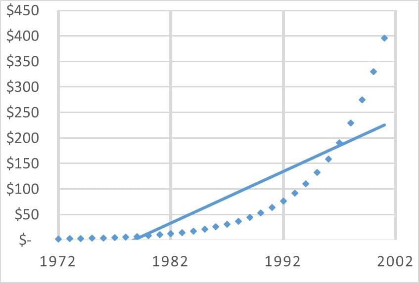
Time-series analysis is a cornerstone of demand forecasting. Moving averages and regression analysis were included at the end of a statistics class that I took years ago. One of my classmates stated that regression analysis appeared complex on the surface, but in reality was simplistic and easy. I agree and disagree. I agree that it is easy to pick two data sets and run the calculation. However, properly specifying and appropriately modeling the data isn’t always so easy. Many of the most common specification and modeling problems can be identified by analyzing the regression’s error terms (how the estimate varies from the data points). One mistake I have made in the past is the use of linear regression to model non-linear trends. This is an example of a mistake that becomes apparent when viewing a plot of the error terms.

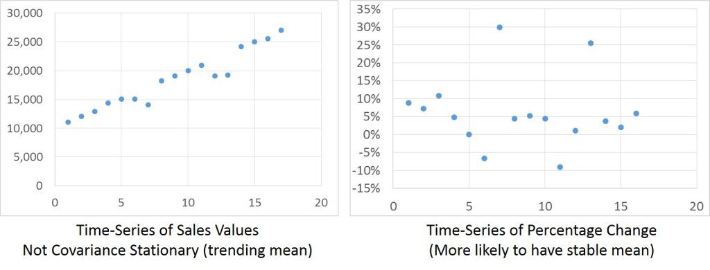
Autoregressive (AR) time-series are a commonly used statistical tool for modeling future demand.  These models use past demand data as independent values to predict future demand as the dependent variable. A basic example of an AR model is the estimation of next quarter’s sales for a given product as a function of the prior quarter’s sales. The quarter-to-quarter relationship would be based on the quarterly data for a number of periods. However, it is a common mistake to use actual sales values as the independent variable. Doing so will produce erroneous results. These models should be designed with a data set that has a stable mean and variance across the time series (no discernable growth or contraction). To properly model a trending time series, try using the change in sales values between periods as the independent variable, rather than the sales values themselves. Doing so will change the independent variables from an absolute quarterly sales value (such as $22,000) to a month to month growth rate ($2,000). At the same time, the mean will change from an average quarterly sales number to an average quarterly growth in sales. When viewing the data plot, you will likely notice that the values will be more evenly distributed across the estimated value (regression line).  Finally, seasonality is a common attribute to demand patterns. Once an autoregressive model has been transformed to remove growth trends, a seasonal lag can often be included as an additional variable to capture and predict seasonality.

Final Thoughts
Supply chain planning software vendors offer some of the most robust demand planning functionality available on the market. The solutions include a broad array of forecasting methods and algorithms, as well as data cleansing and management features. The planning software vendors are consistently improving their solutions by adding features and enhancing the usability of their systems. These usability enhancements streamline processes and minimize complexity by providing step-by-step guidance to the demand planners, allowing them to focus on the big picture. I believe these usability enhancements improve the value of the solutions. But I also believe that it is important to periodically “look under the hood” of the demand planning vehicle being driven.